

Lessons Learned from Winning the RecoGym Challenge
Written by Olivier Jeunen and Bart Goethals, January 31st 2020
Every year around the end of September, the ACM Conference on Recommender Systems (RecSys) is organised. RecSys is the “premier international forum for the presentation of new research results, systems and techniques in the broad field of recommender systems”. Its latest edition, held in Copenhagen, Denmark, attracted over 900 participants from various backgrounds in academia and industry.
In conjunction with the conference, a wide array of workshops are organised as well. Each workshop dives deeper into a specific subfield of RecSys, providing an exciting breeding ground for novel research directions and ideas. The REVEAL workshop held in Vancouver 2018 was one such an event. It focused on the offline evaluation of recommender systems, presenting an admirable line-up of invited speakers and research papers presented in the form of talks or posters. In Copenhagen, the second edition of the REVEAL workshop continued its success, focusing on causality, robust estimators, and the overlap between Reinforcement Learning (RL) and RecSys.
One consensus about current evaluation practices was clear. If we want to talk about recommendation systems as learning interventional policies, we will need interventional data to learn from and evaluate on. This means we need carefully logged datasets with information pertaining to the recommendations that were shown to the users, and the interactions that occurred (or didn’t) as a consequence of the system taking a specific action. The currently most often used datasets in the field (MovieLens, Netflix, Million Song Dataset, LastFM, Yahoo, Jester, …) are lacking in that sense [1]. Furthermore, the datasets that do include this information, can still be insufficient due to the inherent variance that comes with counterfactual estimators. As such, these datasets may provide all the information we need to learn a great recommender, but being able to say with certainty that algorithm A is statistically signficantly better than algorithm B can still be troublesome [2].
In the RL community, the use of simulators is a widely accepted workaround for this inconvenience [3]. Various simulators are available on the OpenAI Gym website for problems ranging from classical control theory to Atari 2600 games. It is with this in mind, that the Criteo AI Lab presented RecoGym at REVEAL 2018 [4]. By simulating both the organic and bandit behaviour of users, RecoGym provides a unified framework for working with and combining classical recommendation algorithms and more recent bandit-based approaches. Additionally, it provides functionality to simulate online experiments such as A/B-tests, which entails further advantages (e.g. you can always simulate more users in your A/B-test, so statistical significance issues are in your own hands).
To encourage and instigate research on this meeting point of RL, counterfactual inference and recommender systems, Criteo announced the RecoGym Challenge at REVEAL 2019. For a certain fixed simulation environment, the goal of participants would be to design a recommendation agent that would beat all others in an A/B test. To ensure generalisability, the final results would come from a thorough evaluation averaged over multiple random seeds and large numbers of test users. To ensure competitivity and practicality of the final submitted solutions, the maximally allowed training time was limited, as well as the amount of available training data your agent starts off with.
In the context of the MSc-level Artificial Intelligence Project course at the University of Antwerp, we teamed up to try our hand at this. In the end, we won the grand prize of €3.000. This blog-post provides an overview of our journey, including stuff that didn’t work, stuff that was promising, and our final solution. We will start off by formalising some notation and clarifying the exact problem set up, and provide an overview of the actual work-horse that is RecoGym’s simulator.
In alphabetical order, the students that participated in the course and the challenge were:
- Nadezhda Avramoska
- Ilion Beyst
- Cedric De Schepper
- Benoît-Phillipe Fornoville
- Tim Hellemans (PhD student)
- Ken Mendes
- Simone Monti
- Gianluca Puleri
- Alp Tunçay
- Benjamin Vandersmissen
Notation and Problem Setup
Typically, recommender systems (and specifically collaborative filtering) research focuses on having a dataset consisting of implicit feedback. For sets of users $\mathcal{U}$ and items $\mathcal{I}$, the set $\mathcal{P} \subseteq \mathcal{U} \times \mathcal{I}$ describes a bipartite mapping between them. A pair $(u,i) \in \mathcal{P}$ then implies that user $u$ has in some way consumed item $i$, be it through a view, a click, a purchase, a streaming event or otherwise. This set $\mathcal{P}$ is often represented as a sparse binary matrix $\mathbf{P} \in {0,1}^{|\mathcal{U}|\times |\mathcal{I}|}$, called the user-item matrix. Generally speaking, this matrix is fed into an algorithm that then tries to learn some inherent general structure of the matrix, in order to be able to predict the most likely missing values in that matrix. Many different methods have been proposed to tackle this problem, where some of the most notable are neighbourhood-based models [5,6], latent factor models [7], linear regression models [8,10], and more recently those based on (variational) auto-encoders [9,10].
It has been argued that this type of interpretation of the recommendation problem can be very different from the objectives of actual recommenders deployed in the wild [11,12]. Instead of purely focusing on this organic user behaviour data, we could look how users actually interact with recommendations. As this strongly relates to (simplified) RL methods such as multi-armed and contextual bandits, this is aptly called bandit feedback. Figures 1 and 2 further clarify this distinction.
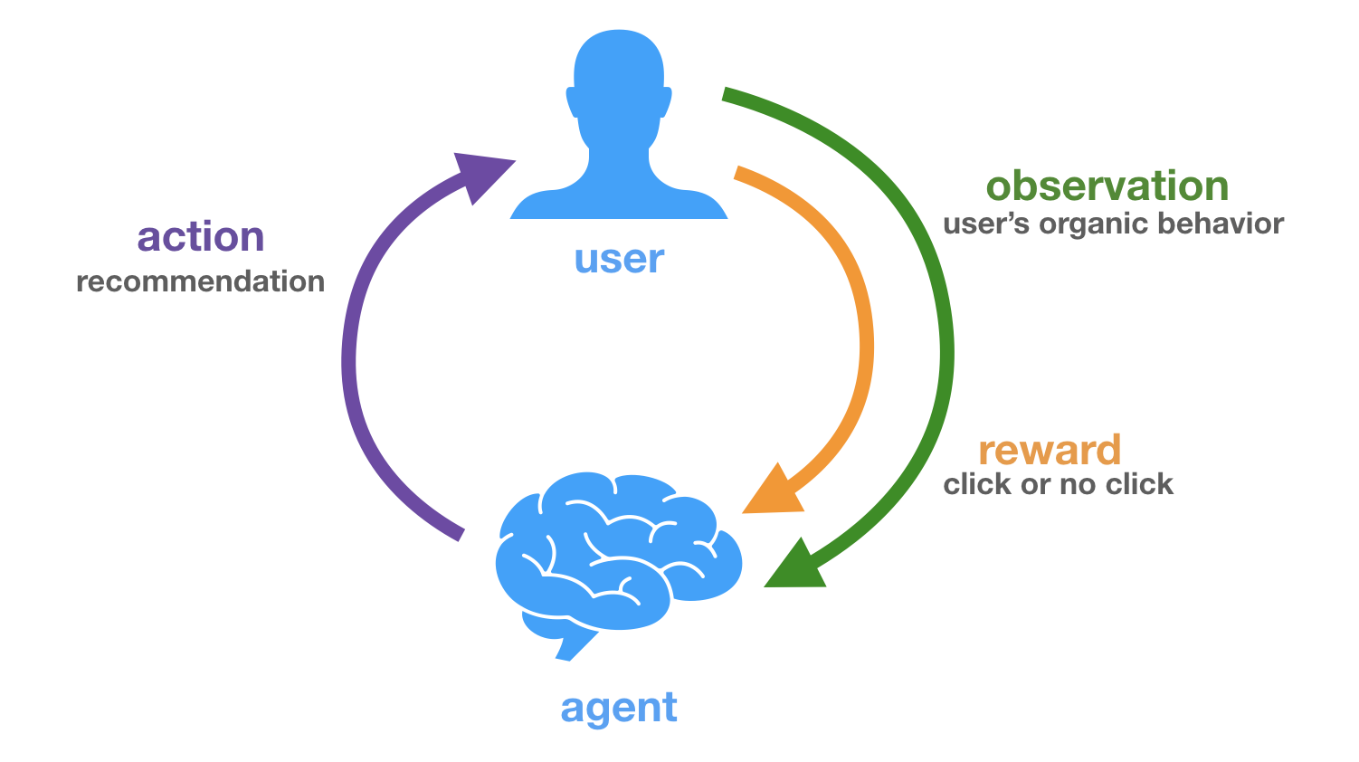
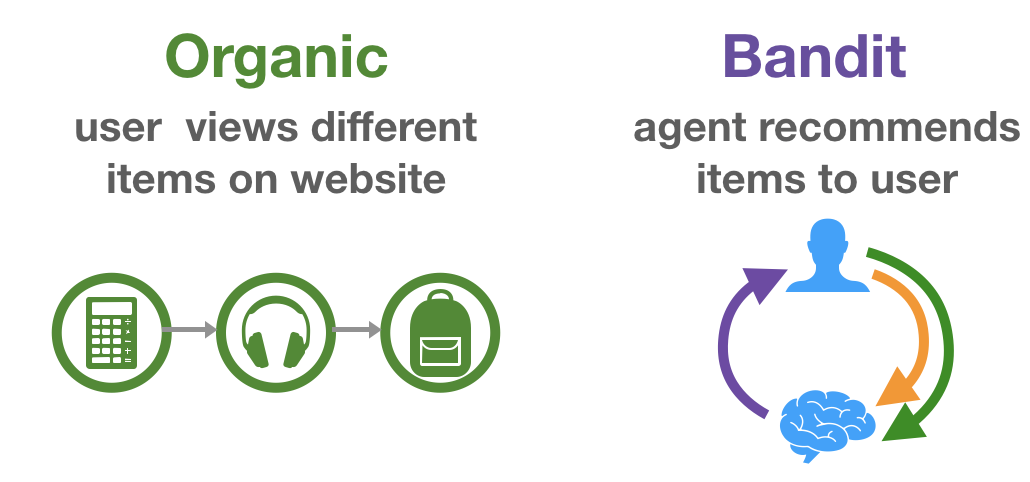
A dataset of logged bandit feedback $\mathcal{D}$ consists of tuples $(\mathbf{x}, a, p, c)$. Generally speaking, this data has been collected under some stochastic logging policy $\pi_0$ that describes a probability distribution over actions (recommendations), conditioned on some context (user history). This policy $\pi_0$ can be seen as a previous version of the production system, more specifically the one that was in place at the time the data was collected. Here, $\mathbf{x} \in \mathbb{R}^n$ describes the user state or context vector. This vector can be of arbitrary dimension and hold any type of information, these are effectively the features that $\pi_0$ looked at to decide which action it should take ($a$) and with which probability ($p \equiv \pi_0(a|\mathbf{x})$). A context-vector $\mathbf{x}$ relates to a user in $\mathcal{U}$, and an action identifier $a$ to an item in $\mathcal{I}$. The observed reward (whether the user interacted with the presented recommendation) is represented as $c \in {0,1}$. RecoGym deals with a binary and direct reward (i.e. click or no click), but many of the covered methods are more generally applicable.
So, we have access to logs of organic behaviour $\mathcal{P}$ as well as bandit behaviour $\mathcal{D}$. At evaluation time, we will observe organic behaviour and select which action to perform (recommendation to show) ourselves. The final evaluation metric is the Click-Through-Rate (CTR) an agent can attain during a simulated A/B-test.
Most of the existing literature in the recommender systems field does not explicitly acknowledge this distinction, but we believe it to be inherent to many real world use-cases.
The Simulator
In what follows, we provide an overview of the actual simulation framework behind RecoGym. Note: we did not write the simulator. Any and all merit should go to the authors of the original paper [4]. We merely aim to provide a comprehensive overview of its inner workings.
RecoGym adopts a latent factor model of user behaviour, as widely accepted in the literature [7]. When the environment is set up, the system generates an embedding consisting of $K$ latent factors for every item. These embeddings are represented in a real-valued matrix $\Gamma \in \mathbb{R}^{|\mathcal{I}|\times {K}}$ and drawn from a multivariate Gaussian distribution centred around 0 with unit variance:
\[\Gamma \sim \mathcal{N}(0,1).\]A notion of item popularity is modelled as an additive bias per item: $\mu \in \mathbb{R}^{|\mathcal{I}|}$ , normally distributed with a configurable variance:
\[\mu \sim \mathcal{N}(0,\sigma_\mu^2).\]$\Gamma$ and $\mu$ directly impact how users organically interact with these items. The RecoGym authors argue that bandit behaviour for an item would be different, but similar to the organic behaviour for a given item. The rationale being that users’ natural browsing behaviour and reactions to recommendations are related, but not an exact one-to-one mapping. As such, bandit embeddings and popularities are obtained by performing a transformation $f$ on the organic parameters:
\[\Xi, \mu' = f(\Gamma, \mu).\]We will not go further in-depth on how this transformation $f$ is performed, as it is of marginal importance for the purposes of this blogpost. Interested readers are referred to the Reco-Gym source code. 1
Users are described by vectors that conceptually reside in the same latent space as the items. That is, a user embedding $\omega \in \mathbb{R}^{K}$ is sampled from a multivariate Gaussian distribution with configurable variance:
\[\omega \sim \mathcal{N}(0,\sigma_u^2).\]Users are simulated sequentially and independently. The behaviour of a single user is modelled as a Markov chain, being either in an “organic” (O) or “bandit” state (B). Figure 3 visualises this process for clarity. The organic state implies the user is currently browsing the item catalog, and generates interactions $(u,i) \in \mathcal{P}$. The bandit state on the other hand requires interventions from the agent, and generates samples $(\mathbf{x},a,p,c) \in \mathcal{D}$.

Organic Views
The next item a user views organically is sampled from a categorical distribution, where the individual probabilities for every item are proportional to how similar the user and the respective item’s latent organic embeddings are. Formally, given $u$, we draw $ i \sim \text{Categorical}(\rho)$ where
\[\rho_i \propto \omega^{\intercal} \Gamma_{i,\cdot} + \mu_i.\]Bandit Feedback on Recommendations
When an action is performed by the agent, the probability of it actually leading to a click is Bernoulli-distributed, with the probability of success being dependent on the similarity between the user and the recommendation’s bandit embedding:
\[c \sim Bernoulli(p) ,\] \[p \propto \omega^{\intercal} \cdot \Xi_{a,\cdot} + \mu_a'.\]Naturally, consistently taking the action $a^*$ with the highest probability of leading to a click leads to an optimal recommendation policy.
\[a^* = \text{arg}\max\limits_{a}(\omega^{\intercal} \cdot \Xi_{a,\cdot} + \mu_a')\]Training Data and the Logging Policy
The table below shows the settings that were fixed for the evaluation of the competition.
| Parameter | Value |
|---|---|
| # Items | 100 |
| # Train users | 1000 |
| # Test users | 10000 |
| # Latent factors | 5 |
| Variance user state | 0.1 |
| Variance item pop. | 3 |
Naturally, when the training data is being generated, some agent needs to choose which actions to actually take. That is, which items to gather feedback for. This agent is often referred to as the logging policy, or $\pi_0$.
The logging policy that generated training data for the challenge was based on a stochastic baseline algorithm that only focuses on the organic data.
It recommends items proportional to how often they have appeared in the users organic item views.
In the context of online advertising, this makes sense: the user has already shown interest in that given item, so advertising it more often sounds reasonable.
If we assume the user state $\mathbf{x} \in \mathbb{R}^{|\mathcal{I}|}$ to be a bag-of-words representation of the user $u$’s organic viewing behaviour, it can be formalised as follows:
It is interesting to note that this logging policy does not have support over the entire action space $\mathcal{I}$. This implies that certain $(\mathbf{x},a)$ combinations will never occur in the training data as $\pi_0(a|\mathbf{x}) = 0$. Many counterfactual learning approaches make use of importance sampling or Inverse Propensity Scoring (IPS). The assumptions needed for importance sampling to provide an unbiased estimator do not hold in this setting.
Methods
We tried our hand at various different approaches to try and tackle the problem. In the rest of this Section, we introduce and discuss them.
Classical Recommendation Approaches
As we have mentioned earlier, many traditional methods for recommendation only take into account organic information. Or at least, they do not explicitly discriminate between different types of interactions, or whether they originated from a system intervention.
Nearest-neighbour and matrix factorisation methods are essential to traditional recommendation research, so they seemed like a good place to start. We looked into traditional item-item models using cosine similarity [5], singular value decomposition [7], and others. Whilst these methods provide strong baselines, it became clear rather quickly that not using the valuable information that is embedded in the bandit feedback would be detrimental.
Matrix factorisation methods could theoretically be extended to exploit both organic and bandit feedback, for example, by regularising the objective (e.g. $l_2$-norm) with something related to the bandit data (e.g. cross-entropy). We did not look into this much further.
Neighbourhood-based methods can be extended rather straightforwardly to take bandit data into account as well. We experimented with a model that looked at a given users’ nearest neighbour users based on organic data, and subsequently used information on these neighbours’ bandit behaviour to decide what to recommend, similar in fashion to the model presented in [13]. Surprisingly, a version of this model that learned online from additional interactions gathered during the A/B-test performed very well, and was our third-best submission.
Value Learning
Focusing entirely on the bandit data, one might want to model the probability of a certain context-action pair leading to a click. Formulating the problem this way makes it clear that we are dealing with a classification problem. As we mentioned earlier, the model that can estimate this quantity the best, and thus always recommend the item with the highest probability of receiving a click, will be the optimal agent. The main issues here are that: (1) the training sample is very limited, and (2) the training sample is extremely skewed as a result of the logging policy picking its actions non-uniformly-at-random.
First, this means we need some way to encode the user state and the action as features. We decided to encode users as bag-of-word vectors over their organic item views. An item $a$ can be one-hot-encoded into $\mathbf{a} \in {0,1}^{|\mathcal{I}|}$. Simply concatenating these vectors $\mathbf{x}$ and $\mathbf{a}$ would not allow for personalisation in a linear model. To obtain second-order features, we adopt the Kronecker-product: $(\mathbf{x} \otimes \mathbf{a}) \in \mathbb{R}^{|\mathcal{I}|^2}$. Because $\mathbf{a}$ is sparse, so is $(\mathbf{x} \otimes \mathbf{a})$. SciPy provides many ways of efficiently dealing with sparse matrices [14].
Many out-of-the-box classifiers exist and are widely available to model the probability of a click:
\[P(C | \mathbf{x}, a).\]We looked into logistic regression, naive Bayes, random forests, gradient-boosted trees, multilayer perceptrons et cetera. All were able to provide models with decent performance, but the gains from more advanced algorithms were marginal. The main reason for this is that since the training sample was that limited, more complex models would become much more prone to overfitting.
Additionally, we looked into more advanced ways of modelling the context-action pairs. As the number of items $|\mathcal{I}|$ grows, the quadratic nature of the Kronecker product might become prohibitive. Auto-encoders gave us promising results in this direction.
Policy Learning
In the end, modelling whether a context-action pair will lead to a click is only a rest stop on the road to getting more clicks. We might want to directly model a policy $\pi(a|\mathbf{x})$, mapping contexts to actions:
\[P(A | \mathbf{x}).\]This type of model can be optimised in many ways. The most common is to define some estimator $\mathcal{R}(\pi,\mathcal{D})$ of the reward that the policy $\pi$ can obtain, based on a dataset of logged bandit feedback $\mathcal{D}$. An empirical IPS estimator can be defined as follows:
\[\widehat{\mathcal{R}}(\pi,\mathcal{D}) = \frac{1}{\mathcal{D}} \sum_{(\mathbf{x},a,p,c) \in \mathcal{D}}c\frac{\pi(a|\mathbf{x})}{\pi_0(a|\mathbf{x})}.\]Theoretically, the parameters of the policy $\pi$ could then be optimised via gradient ascent to optimise this estimator. This is the cornerstone of counterfactual inference, and has been specifically investigated with an application to computational advertising by Bottou et al. [16]. Furthermore, it’s closely related to policy gradient algorithms such as REINFORCE [17], which have in turn been recently linked to recommender systems use cases [18]. In the RecoGym setting, we only care about immediate rewards, top-1 recommendation and logging propensities are known. This makes policy gradient algorithms such as REINFORCE equivalent to the work of Bottou, as they just provide another way to optimize the reward estimate.
In general, these policy-based methods tend to perform better than their value-based counterparts when the training sample is limited. However, as we mentioned earlier, the logging policy does not adhere to the assumptions necessary for the IPS estimator to be unbiased. Additionally, the variance of these estimators can often grow to be prohibitively large, skewing the estimates even further. We refer the interested reader to the work of Swaminathan and Joachims [20] and their more recent works for more methods to deal with the Batch Learning from Bandit Feedback (BLBF) setting we encounter here. For a general comparison between value- and policy-based methods for training models on bandit feedback, see [19].
Online Bandits
It is clear that for both the value- and policy-based approaches, the limited training sample can be problematic. Because of this, we decided to look into contextual bandit approaches that can learn online during the A/B-test and handle the exploration-exploitation trade-off in an efficient and effective manner.
To start off, we looked at an $\epsilon$-greedy batch-based approach: with probability $\epsilon$ perform an action uniformly at random, otherwise perform the action for which the estimate $P(C = 1| \mathbf{x}, a)$ is highest. As the number of test users is set to be considerably higher than the number of training users (in order to ensure statistical significance of the A/B-test results), it became clear rather quickly that there was much to be gained by adopting online learning methods.
As $\epsilon$-greedy approaches are a rather naive way of dealing with explore-exploit, we decided to delve into methods that can handle this in a more principled manner. We looked into upper-confidence-bound based approaches such as LinUCB [21] and Thompson sampling-based methods such as the one proposed by Chapelle and Li [22] and in [23]. Although these methods are tried and true, getting them to perform properly in our experimental set-up was non-trivial. The update steps in all of them require a matrix inversion, which made it infeasible to update the model parameters after every action. Furthermore, initialising the model parameters sensibly from the training data was not straightforward either, as it was skewed towards the logging policy.
Overall, results were very promising, but highly variable over different runs.
The Winning Solution
Discriminative models have been shown to be effective learners, certainly when the training sample is large. Generative models, on the other hand, can often perform better in small data regimes [24]. Our final solution was based on a generative naive Bayes classifier where we assume a multinomial distribution over features and a uniform prior [25]. This Section will discuss the specifics of our methodology. For notational simplicity, we will denote the Kronecker-product between the action- and user-specific features as $\mathbf{X} \equiv \mathbf{x} \otimes \mathbf{a}$.
Bayes’ theorem states the following:
\[P(C = 1 | \mathbf{X}) = \frac{P(C = 1) P(\mathbf{X} | C = 1)}{P(\mathbf{X})} .\]Naively assuming conditional independence between the features, gives us
\[P(C = 1 | \mathbf{X}) = \frac{P(C = 1) \prod_{i = 0}^{|\mathcal{I}|^2 } P(\mathbf{X}_i|C = 1)}{P(\mathbf{X})} .\]As the quantity $P(X)$ can be seen as a constant here, we can drop it and approximate the probability of receiving a click as
\[P(C = 1 | \mathbf{X}) \propto P(C = 1) \prod_{i = 0}^{|\mathcal{I}|^2 } P(\mathbf{X}_i|C = 1).\]We can gather estimates for the click prior and these conditional probabilities through Maximum Likelihood Estimation (MLE) on the training sample, yielding
\[\widehat{P}(C = 1) = \frac{\sum_{(\mathbf{x},a,p,c) \in \mathcal{D}}c}{|\mathcal{D}|} \text{, and } \widehat{P}(\mathbf{X}_i| C = 1) = \frac{ \sum_{(\mathbf{x},a,p,c) \in \mathcal{D}}c\mathbf{X}_i}{ \sum_{(\mathbf{x},a,p,c) \in \mathcal{D}} \sum_{j = 0}^{|\mathcal{I}|^2}c\mathbf{X}_j}.\]Such models are often used baselines in text classification, where a bag-of-words representation is used to represent documents instead of users. Now, the main issue that remains is that the conditional probability estimate for a feature $\mathbf{X}_i$ will be zero if it never occurred in the training sample. Additionally, the training sample is severely biased due to the logging policy being highly selective with its actions, and not having support over the entire action space for every context. Because of this, most $(\mathbf{x},a)$-combinations will never occur in the limited training sample, and many $\mathbf{X}_i$’s will always be zero. Naturally, the conditional probabilities $\widehat{P}(\mathbf{X}_i| C = 1)$ will be too.
This can be alleviated through additive smoothing, i.e. adding a pseudo-count $\alpha$ to the observations. From a probabilistic point of view, we incorporate a prior belief that features $\mathbf{X}_i$ occur uniformly regardless of whether a click has occurred:
\[\widehat{P}(\mathbf{X}_i| C = 1) = \frac{ \sum_{(\mathbf{x},a,p,c) \in \mathcal{D}}c(\mathbf{X}_i+\alpha)}{ \sum_{(\mathbf{x},a,p,c) \in \mathcal{D}} \sum_{j = 0}^{|\mathcal{I}|^2}c(\mathbf{X}_j+\alpha)}.\]This hyperparameter $\alpha$ can be optimised through a cross-validated grid search on the training sample, and it proved to be a crucial element contributing to the performance of the approach. One of the biggest advantages of the naive Bayes approach is that the model can be incrementally trained as new samples come in very easily. As $\mathcal{D}$ grows, the empirical probability estimates are updated to reflect the new information. Because the training sample is extremely limited and the number of test users in the A/B test is large to ensure statistically significant results, the benefits from online learning are not to be underestimated. Furthermore, we can explore $(\mathbf{x},a)$-regions that the logging policy didn’t, and hope to close in on a better reward estimator. Note that we do not incorporate any explicit notion of exploration such as $\epsilon$-greedy, but that exploration is implicitly incentivised through the uniform prior.
When the environment asks the agent to perform an action given $\mathbf{x}$, it performs the action it deems most likely to lead to a click (ties are broken at random):
\[a^{*} = \text{arg}\max\limits_{a}\prod_{i = 0}^{|\mathcal{I}|^2 } \widehat{P}((\mathbf{x}\otimes\mathbf{a})_i|C = 1).\]One final insight that boosted performance further was that the pseudocounts $\alpha$ bring the biggest advantage when there’s a lot of uncertainty, i.e. at the beginning of the experimental runs, when the amount of data is relatively low and many $(\mathbf{x},a)$-pairs unexplored. Annealing the effect of the prior through this parameter as more and more training data came in, resulted in a consistent improvement.
Conclusion
In this blogpost, we presented an overview of our journey participating in the RecoGym Challenge organised by Criteo. We discussed shortcomings of classical approaches to recommendation, difficulties with more advanced policy learning methods and contextual bandits, and introduced our solution based on an incrementally retrained naive Bayes classifier with an annealed pseudo-count.
We would like to stress once again that this was a team achievement, and thank the participating students for their hard work and effort. Additionally, we thank the organisers at Criteo for setting up the competition, and hope this can spark further research at the intersection of RL, counterfactual interference and recommendation systems.
References
[1] Jeunen, Olivier. “Revisiting offline evaluation for implicit-feedback recommender systems.” Proceedings of the 13th ACM Conference on Recommender Systems. 2019.
[2] Lefortier, Damien, et al. “Large-scale validation of counterfactual learning methods: A test-bed.” arXiv preprint arXiv:1612.00367 (2016).
[3] Brockman, Greg, et al. “OpenAI Gym.” arXiv preprint arXiv:1606.01540 (2016).
[4] Rohde, David, et al. “Recogym: A reinforcement learning environment for the problem of product recommendation in online advertising.” arXiv preprint arXiv:1808.00720 (2018).
[5] Sarwar, Badrul, et al. “Item-based collaborative filtering recommendation algorithms.” Proceedings of the 10th international conference on World Wide Web. 2001.
[6] Verstrepen, Koen, and Bart Goethals. “Unifying nearest neighbors collaborative filtering.” Proceedings of the 8th ACM Conference on Recommender systems. 2014.
[7] Koren, Yehuda, Robert Bell, and Chris Volinsky. “Matrix factorization techniques for recommender systems.” Computer 42.8 (2009): 30-37.
[8] Ning, Xia, and George Karypis. “SLIM: Sparse linear methods for top-n recommender systems.” 2011 IEEE 11th International Conference on Data Mining. IEEE, 2011.
[9] Liang, Dawen, et al. “Variational autoencoders for collaborative filtering.” Proceedings of the 2018 World Wide Web Conference. 2018.
[10] Steck, Harald. “Embarrassingly shallow autoencoders for sparse data.” The World Wide Web Conference. 2019.
[11] Jeunen, Olivier, et al. “Learning from Bandit Feedback: An Overview of the State-of-the-art.” arXiv preprint arXiv:1909.08471 (2019).
[12] Jeunen, Olivier, David Rohde, and Flavian Vasile. “On the Value of Bandit Feedback for Offline Recommender System Evaluation.” arXiv preprint arXiv:1907.12384 (2019).
[13] Nguyen-Thanh, Nhan, et al. “Recommendation System-based Upper Confidence Bound for Online Advertising.” arXiv preprint arXiv:1909.04190 (2019).
[14] Bressert, Eli. SciPy and NumPy: an overview for developers. “ O’Reilly Media, Inc.”, 2012.
[15] Owen, Art. Monte Carlo Theory, Methods and Examples. 2013.
[16] Bottou, Léon, et al. “Counterfactual reasoning and learning systems: The example of computational advertising.” The Journal of Machine Learning Research 14.1 (2013): 3207-3260.
[17] Williams, Ronald J. “Simple statistical gradient-following algorithms for connectionist reinforcement learning.” Machine learning 8.3-4 (1992): 229-256.
[18] Chen, Minmin, et al. “Top-k off-policy correction for a REINFORCE recommender system.” Proceedings of the Twelfth ACM International Conference on Web Search and Data Mining. 2019.
[19] Mykhaylov, Dmytro, et al. “Three Methods for Training on Bandit Feedback.” arXiv preprint arXiv:1904.10799 (2019).
[20] Swaminathan, Adith, and Thorsten Joachims. “Counterfactual risk minimization: Learning from logged bandit feedback.” International Conference on Machine Learning. 2015.
[21] Li, Lihong, et al. “A contextual-bandit approach to personalized news article recommendation.” Proceedings of the 19th international conference on World wide web. 2010.
[22] Chapelle, Olivier, and Lihong Li. “An empirical evaluation of thompson sampling.” Advances in neural information processing systems. 2011.
[23] Dumitrascu, Bianca, Karen Feng, and Barbara Engelhardt. “PG-TS: Improved Thompson sampling for logistic contextual bandits.” Advances in neural information processing systems. 2018.
[24] Ng, Andrew Y., and Michael I. Jordan. “On discriminative vs. generative classifiers: A comparison of logistic regression and naive bayes.” Advances in neural information processing systems. 2002.
[25] Manning, Christopher D., Prabhakar Raghavan, and Hinrich Schütze. Introduction to information retrieval. Cambridge university press, 2008.
-
The original code uses $B$ instead of $\Xi$, we decided to change this to avoid confusion with the bandit state in the Markov chain representing user behaviour. ↩